Imaging Tutorial

In this tutorial, we will see how to obtain calibrated images and light curves from a set of on-the-fly (OTF) scans done with the SRT. Data are taken with the SARDARA ROACH2-based backend, with a bandwidth of 1024 MHz and 1024 channels. In this tutorial we will first learn how the software does a semi-automatic cleaning of the data from radio-frequency interferences (RFI), and how to tweak the relevant parameters to do the cleaning properly. Then, we will generate rough images with the default baseline subtraction algorithms. Afterwards, we will load a set of calibrators to perform the conversion from signal level to Janskys/pixel. Finally, we will apply the calibration to the previously generated images.

Note

If you are using Anaconda: remember to initialize the environment. E.g. for an environment called py3

$ source activate py3

Inspect the observation

During a night of observations, we will in general observe a number of calibrators and sources, in random order. Our observation will be split into a series of directories:

(py3) $ ls
2016-05-04-220022_Src1/
2016-05-04-223001_Src1/
2016-05-04-230001_Cal1/
2016-05-04-230200_Cal2/
2016-05-04-230432_Src1/
2016-05-04-233523_Src1/
(....)

Some of these observations might have been done in different bands, or using different receivers, and you might have lost the list of observations (or the user was not the observer). The script SDTinspect is there to help, dividing the observations in groups based on observing time, backend, receiver, etc.:

(py3) $ SDTinspect */
Group 0, Backend = ROACH2, Receiver = CCB
------------------
Src1, observation 0

Source observations:
2016-05-04-220022_Src1/
2016-05-04-223001_Src1/
2016-05-04-230432_Src1/

Calibrator observations:
2016-05-04-230001_Cal1/
2016-05-04-230200_Cal2/

Group 1, Backend = ROACH2, Receiver = KKG
---------------
Src1, observation 1

Source observations:
2016-05-04-233523_Src1/
(.....)

Calibrator observations:
(.....)

With the -d option, the script will also dump automatically a set of config files ready for the next step in the analysis:

(py3) $ SDTinspect */
Group 0, Backend = ROACH2, Receiver = CCB
(.....)
(py3) $ ls -alrt
CCB_ROACH_Src1_Obs0.ini
KKG_ROACH_Src1_Obs1.ini

Note

Many observation schedules add labels to the source name (e.g. _RA or _Dec to indicate scans in a given direction, _K to indicate the band, etc). This is not ideal and should always be avoided. However, to manage this use case it is sufficient to add the option --ignore-suffix to SDTinspect, followed by a list of comma-separated patterns to be avoided. For example, if we want to avoid the suffixes _RA and _Dec we can run

(py3) $ SDTinspect --ignore-suffix _RA,_Dec (... other options)

Modify config files

If you did not pre-generate config files with the procedure above, you can generate a boilerplate config file with:

(py3) $ SDTlcurve --sample-config
(py3) $ ls
(...)
sample_config_file.ini

In the following, we will use the config files generated by SDTinspect, but it is very easy to adapt to the case of a custom-modified boilerplate.

Config files have this overall structure (slight changes might occur, like equals signs being changed to semicolons):

(py3) $ cat CCB_ROACH_Src1_Obs0.ini
[local]
workdir = .
datadir = .

[analysis]
projection = ARC
interpolation = spline
list_of_directories =
    2016-05-04-220022_Src1/
    2016-05-04-223001_Src1/
    2016-05-04-230432_Src1/
calibrator_directories =
    2016-05-04-230001_Cal1/
    2016-05-04-230200_Cal2/
noise_threshold = 5
pixel_size = 1
goodchans =

You will likely not change the kind of interpolation or the projection in the plane of the sky (but if instead of ARC you want something different, all projections in this list are supported). goodchans is a list of channels that can be excluded from automatic filtering (for example, because they might contain an important spectral line.)

pixel_size is by default 1 arcminute. You might want to change this depending on the density of scans and the beam size at the observing frequency. Usually, 1/3 of the beam size is ok for dense OTF scan campaigns, while a larger value is better for sparse observations.

Also, you might know already that some observations were bad. In this case, it’s sufficient to take them out of the list above.

Preprocess the files

Figure 2. Output of the automatic filtering procedure for an OTF scan of a calibrator. Channels where the root mean square of the signal is too high or too low are automatically filtered out. The threshold is encoded in the noise_threshold variable in the config file. This is the number of standard deviations from the median r.m.s. in a given interval. Optionally the user can choose the frequency interval (blue vertical lines). In the two right panels, one can see the scan before and after the cleaning. In the right-lower panel, the uncleaned scan is reported in grey to help the eye. The dynamical spectrum before and after the cleaning is shown in the two middle panels, and the effect of the cleaning on the scan is shown in the two right panels

This step is optional, because it can be merged with image production. However, for the sake of this tutorial we will proceed in this way for simplicity.

The easiest way to preprocess an observation is to call SDTpreprocess on a config file. The script will load all files, one by one, and do the following steps:

1. If the backend is spectroscopic, load each scan and filter out all channels whose that are more noisy than a given value of rms during the scan, then merge into a single channel. As an option (recommended), the user can specify a frequency interval that will be merged, otherwise the full frequency interval is taken: for this, one can use the option --splat <minf:maxf> where minf, mmaxf are in MHz referred to the minimum frequency of the interval. E.g. if our local oscillator is at 6900 MHz and we want to cut from 7000 to 7500, minf and mmaxf will be 100 and 600 resp. This process produces plots like the following:

(py3) $ SDTpreprocess -c CCB_TP_Src1_Obs0.ini --splat 80:1100 <more options>

2. About the <more options>>: If you select the option * ``–sub``, the single channels that are produced at step 1, or alternatively the single channels of a non-spectroscopic backend, will now be processed by a baseline subtraction routine. This routine, by default, applies an Asymmetric Least Squares Smoothing (`Eilers and Boelens 2005`_) to find the rough alignment of the scan, and then improves it by selecting the data that are closer to the baseline and making a standard least-square fit. This procedure is very fast and aligns the vast majority of scans in a fraction of a second. For more complicated scans, an interactive interface is also available, albeit with some portability issues that will be solved in future versions (use the ``–interactive`` option). It is possible to avoid regions with known strong sources. For now, they need to be specified by hand, with the ``-e`` option followed by a valid ds9-compatible region file containing *circular regions in the fk5 frame.

3. The results of the first points are saved as HDF5 files in the same directory as the original fits files. This makes it much faster to reload the scans for further use. If the user wants to reprocess the files from scratch, they need to delete these files first, or select the --refilt option.

Let’s produce some images now!

Finally, let us execute the map calculation. If data were taken with a Total Power-like instrument and they do not contain spectral information, it is sufficient to run

(py3) $ SDTimage -c CCB_TP_Src1_Obs0.ini --sub

where CCB_TP_Src1_Obs0.ini should be substituted with the wanted config file. This is also valid for spectroscopic scans that have already been preprocessed

(py3) $ SDTimage -c CCB_ROACH_Src1_Obs0.ini --sub

Otherwise, if preprocessing were not executed before, specify the minimum and maximum frequency to select in the spectrum, with the --splat option (same as before)

(py3) $ SDTimage -c CCB_ROACH_Src1_Obs0.ini --splat <freqmin>:<freqmax> --sub

The above command will:

• Run through all the scans in the directories specified in the config file

• Clean them up if not already done in a previous step, in the same way of SDTpreprocess, including the baseline subtraction algorithm.

• Create a single frequency channel per polarization by summing the contributions between freqmin and freqmax, and discarding the remaining frequency channels, again if not already done in a previous step;

• Create the map in FITS format readable by DS9. The FITS extensions IMGCH0, IMGCH1, etc. contain an image for each polarization channel. The extensions IMGCH<no>-STD will contain the error images corresponding to IMGH<no>.

Note

When the user wants to reprocess the data from scratch, they have to remember the --refilt option. Otherwise, some steps like the spectral summation and the baseline subtraction are not repeated.

The automatic RFI removal procedure might have missed some problematic scan. The map might have, therefore, some residual “stripes” due to bad scans or wrong baseline subtraction.

The first thing to do, in these cases, is to go and look at the scans (by going through the PDF files produced by the calibration process in each subdirectory) and check that the noise threshold is appropriate for the level of noise found in scans. If it is not, as is often the case, and it is sufficient to re-run SDTpreprocess with the noise threshold changed in the config file to get a better cleaning of the data.

But SDTimage has an additional option to align the scans. It’s called global baseline subtraction. This procedure makes a global fit (option -g) of all scans in an image, and tries to find the alignment of each scan that minimizes the total rms of the image. This procedure is only valid if the region that is fit is consistent with having zero average. This is, of course, not valid if the source is strong. In this case, together with the global fit option, we need to also specify a set of regions to neglect. This is done in two ways:

• through a ds9-compatible region file containing circular regions in image coordinates

• through the option -e followed by multiples of three numbers: X, Y and radius, in image coordinates (SAOimage ds9 or other imaging programs can create regions with these coordinates, one just needs to copy the numbers.).

In summary, to use the global fitting and discard the region centered at coordinates x,y=30,33 with radius 10 pixels, run

(py3) $ SDTimage -g -e 30 33 10 (...additional options)

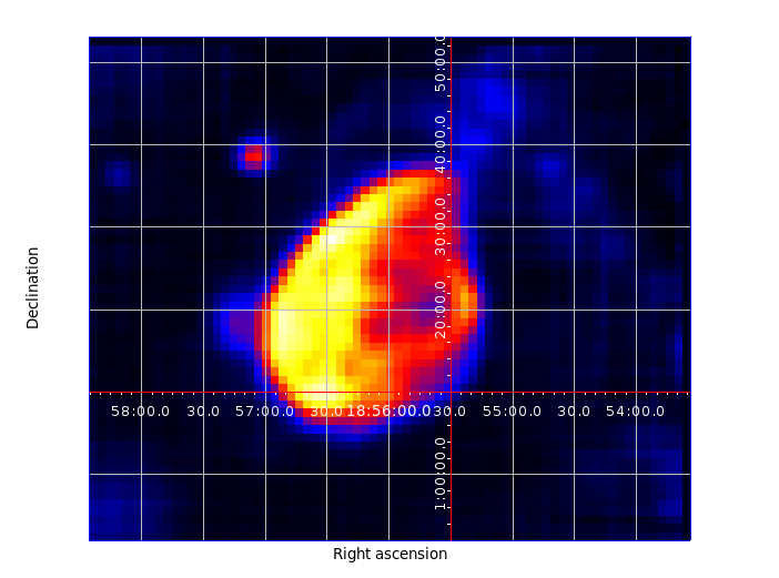
Figure 3. Map produced by SDTimage

Advanced imaging (TBC)

The automatic RFI removal procedure is often unable to clean all the data. The map might have some residual “stripes” due to bad scans. No worries! Launch the above command with the --interactive option

(py3) $ SDTimage -c MySource.ini --splat <freqmin>:<freqmax> --interactive

This will open a screen like this:

<placeholder>

where on the right you have the current status of the image, and on the left, larger, an image of the standard deviation of the pixels. Pixels with higher standard deviation might be due to a real source with high variability or high flux gradients, or to interferences. On this standard deviation image, you can point with the mouse and press ‘A’ on the keyboard to load all scans passing through that pixel. A second window will appear with a bunch of scans.

<placeholder>

Click on a bad scan and filter it according to the instructions printed in the terminal.

Calibration of images

To calibrate the images, one needs to call SDTcal with the same config files used for the images if they were produced with SDTinspect. Otherwise, one can construct an alternative config file with

(py3) $ SDTcal  --sample-config

and modify the configuration file adding calibrator directories below calibrator_directories

calibrator_directories :
   datestring1-3C295/
   datestring2-3C295/

Then, call again SDTcal with the --splat option, using the same frequency range of the sources.

(py3) $ SDTcal -c CCB_ROACH_Src1_Obs0.ini --splat <freqmin>:<freqmax> -o calibration.hdf5

Sometimes, calibrator observations yield bad measurements. The --snr-min option puts a lower limit to the significance of calibration measurements. Finer filtering can be made loading the calibration.hdf5 file into a CalibratorTable or astropy.Table object, and filtering the bad calibratonr measurements by hand. Diagnostics on the calibrator fitting can be found in the data subdirectories (inside directories whose names end in _scandir), and that can also help eliminating bad measurements.

Finally, call SDTimage with the --calibrate option, e.g.

(py3) $ SDTimage --calibrate calibration.hdf5 -c CCB_ROACH_Src1_Obs0.ini --splat <freqmin>:<freqmax> --interactive

… and that’s it! The image values will be expressed in Jy instead of counts, so that applying a region with DS9 and calculating the total flux inside the given region will return the actual total flux contained in the region.

Calibrated light curves

Go to a directory close to your data set. For example

(py3) $ ls
observation1/
observation2/
calibrator1/
calibrator2/
observation3/
calibrator3/
calibrator4/
(....)

It is not required that scan files are directly inside observation1 etc., they might be inside subdirectories. The important thing is to correctly point to them in the configuration file as explained below.

Produce a dummy calibration file, to be modified, with

(py3) $ SDTlcurve --sample-config

This produces a boilerplate configuration file, that we modify to point to our observations, and give the correct information to our program

(py3) $ mv sample_config_file.ini MySource.ini  # give a meaningful name!
(py3) $ emacs MySource.ini

(... modify file...)

(py3) $ cat sample_config_file.ini
(...)
[analysis]
(...)
list_of_directories :
;;Two options: either a list of directories:
    dir1
    dir2
    dir3
calibrator_directories :
    cal1
    cal2
noise_threshold : 5

;; Channels to save from RFI filtering. It might indicate known strong spectral
;; lines
goodchans :

Finally, execute the light curve creation. If data were taken with a Total Power-like instrument and they do not contain spectral information, it is sufficient to run

(py3) $ SDTlcurve -c MySource.ini

Otherwise, specify the minimum and maximum frequency to select in the spectrum, with the --splat option

(py3) $ SDTlcurve -c MySource.ini --splat <freqmin>:<freqmax>

where freqmin, freqmax are in MHz referred to the minimum frequency of the interval. E.g. if our local oscillator is at 6900 MHz and we want to cut from 7000 to 7500, freqmin and freqmax will be 100 and 600 resp. The above command will:

• Run through all the scans in the directories specified in the config file

• Clean them up with a rough but functional algorithm for RFI removal that makes use of the spectral information

• Create a csv file for each source, containing three columns: time, flux, flux error for each cross scan

The light curve will also be saved in a text file.

Sun images

Images of the Sun need only a small change in the processing. During SDTpreprocess and SDTimager, when the user loads data from within 3 degrees of the Sun, Helioprojective coordinates are automatically calculated along with the ICRS and horizontal ones. At this point, to get a map in these coordinates it is sufficient to specify the --frame sun option to SDTimage.

(py3) $ SDTimage -c CCB_TP_Src1_Obs0.ini <other options> --frame sun

This will produce an output file ending with _sun.fits. The correctness of the processing can be quickly tested using SunPy:

import sunpy.map
sunmap = sunpy.map.Map("CCB_TP_Dummy_Obs0_sun.fits")
sunmap.peek()

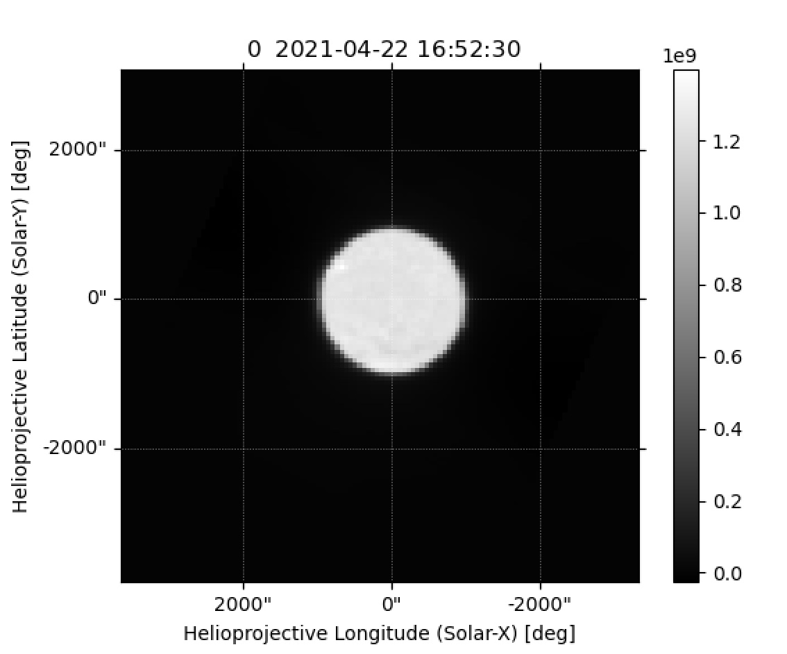
Figure 4. Example Sun observation, plotted with SunPy